Judea Pearl recently wrote a book for a popular audience about his life work, called “The Book of Why”. Pearl is the inventor of “Bayesian Networks”, which are graphs whose links are probabilities. Such a graph might have some nodes that represented symptoms of a disease, and other nodes that represented various diseases. The links between nodes, as well as the decision of which nodes link to which, can help diagnose which disease a person has, given his symptoms. The probabilities propagate using “Bayes Rule”. Despite the huge success of Bayesian Networks, Professor Pearl was not satisfied, so he invented causal networks and a causal language to go with them. This latter discovery has big implications for machine learning.
In what follows, I’ll assume you know Bayes Rule, and I give a flavor of what he accomplished, based on the book.
The weakness of associations in probability are that they don’t tell you what caused what. The rooster may crow just before sunrise, but the association doesn’t tell you whether the approaching sunrise caused the rooster to crow or the rooster’s crowing caused the sunrise.
Lets start with some interesting aspects of Bayesian Graphs.
The simplest Bayes net would be a junction between two nodes that is updated via Bayes Rule. But lets look at junctions that involve 3 nodes (which could exist in a huge graph of hundreds of nodes). The following is a quote from the book:
There are three basic types of junctions, with the help of which we can characterize any pattern of arrows in the network.
1. A -> B -> C. This junction is the simplest example of a “chain,” or of mediation. In science, one often thinks of B as the mechanism, or “mediator,” that transmits the effect of A to C. A familiar example is
Fire -> Smoke -> Alarm.
Although we call them “fire alarms,” they are really smoke alarms. The fire by itself does not set off an alarm, so there is no direct arrow from Fire to Alarm. Nor does the fire set off the alarm through any other variable, such as heat. It works only by releasing smoke molecules in the air. If we disable that link in the chain, for instance by sucking all the smoke molecules away with a fume hood, then there will be no alarm. This observation leads to an important conceptual point about chains: the mediator B “screens off” information about A from C, and vice versa. Suppose we had a database of all the instances when there was fire, when there was smoke, or when the alarm went off. If we looked at only the rows where Smoke = 1 (i.e. TRUE), we would expect Alarm = 1 every time, regardless of whether Fire = 0 (FALSE) or Fire = 1 (TRUE).
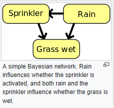
2. A < — B — > C. This kind of junction is called a “fork,” and B is often called a common cause or confounder of A and C. A confounder will make A and C statistically correlated even though there is no direct causal link between them. A good example (due to David Freedman) is Reading Ability.
Children with larger shoes tend to read at a higher level. But the relationship is not one of cause and effect. Giving a child larger shoes won’t make him read better! Instead, both variables are explained by a third, which is the child’s age. Older children have larger shoes, and they also are more advanced readers. We can eliminate this spurious correlation, as Karl Pearson and George Udny Yule called it, by conditioning on the child’s age. For instance, if we look only at seven-year-olds, we expect to see no relationship between shoe size and reading ability.
3. A — > B < — C an example: Talent — > Celebrity < — Beauty. Here we are asserting that both talent and beauty contribute to an actor’s success, but beauty and talent are completely unrelated to one another in the general population. We will now see that this collider pattern works in exactly the opposite way from chains or forks when we condition on the variable in the middle. If A and C are independent to begin with, conditioning on B will make them dependent. For example, if we look only at famous actors (in other words, we observe the variable Celebrity = 1), we will see a negative correlation between talent and beauty: finding out that a celebrity is unattractive increases our belief that he or she is talented. This negative correlation is sometimes called collider bias or the “explain-away” effect. For simplicity, suppose that you don’t need both talent and beauty to be a celebrity; one is sufficient. Then if Celebrity A is a particularly good actor, that “explains away” his success, and he doesn’t need to be any more beautiful than the average person. On the other hand, if Celebrity B is a really bad actor, then the only way to explain his success is his good looks. So, given the outcome Celebrity = 1, talent and beauty are inversely related—even though they are not related in the population as a whole. Even in a more realistic situation, where success is a complicated function of beauty and talent, the explain-away effect will still be present. .The miracle of Bayesian networks lies in the fact that the three kinds of junctions we are now describing in isolation are sufficient for reading off all the independencies implied by a Bayesian network, regardless of how complicated.
Pearl then explains that Bayes Rule lets you update your belief in a hypothesis when new data is presented. It lets you calculate a backward probability, given a forward probability:
Suppose you take a medical test to see if you have a disease, and it comes back positive. How likely is it that you have the disease? For specificity, let’s say the disease is breast cancer, and the test is a mammogram. In this example the forward probability is the probability of a positive test, given that you have the disease: P(test | disease). This is what a doctor would call the “sensitivity” of the test, or its ability to correctly detect an illness. Generally it is the same for all types of patients, because it depends only on the technical capability of the testing instrument to detect the abnormalities associated with the disease. The inverse probability is the one you surely care more about: What is the probability that I have the disease, given that the test came out positive? This is P(disease | test), and it represents a flow of information in the non-causal direction, from the result of the test to the probability of disease. This probability is not necessarily the same for all types of patients; we would certainly view the positive test with more alarm in a patient with a family history of the disease than in one with no such history. Notice that we have started to talk about causal and non-causal directions.
For the next quote, you should understand that we can rewrite Bayes’s rule as follows: (Updated probability of Disease once the test results are in) = P(D | T) = (likelihood ratio) × (prior probability of D) where the new term “likelihood ratio” is given by P(T | D)/P(T).
Judea Pearl was reading about neural network models of the brain, and he put that together with Bayes Rule when he first planned how Bayesian Networks would work.
I assumed that the network would be hierarchical, with arrows pointing from higher neurons to lower ones, or from “parent nodes” to “child nodes.” Each node would send a message to all its neighbors (both above and below in the hierarchy) about its current degree of belief about the variable it tracked (e.g., “I’m two-thirds certain that this letter is an R”). The recipient would process the message in two different ways, depending on its direction. If the message went from parent to child, the child would update its beliefs using conditional probabilities,… If the message went from child to parent, the parent would update its beliefs by multiplying them by a likelihood ratio, as in the mammogram example.
In other words, ‘forward probability’ (Test | Disease) would be passed down, backward probability (Disease | Test) would be passed up.
In image recognition of a word, the probability of a word being “Lion” might be increase by a message passed up to a parent that there is more evidence that the first letter is “L”, and in turn, the more evidence there is for “Lion”, the more probability given to the message passed downward that the first letter is “L”.
So why didn’t Professor Pearl rest on his laurels? He states some limitations with Bayesian networks:
By design, in a Bayesian network, information flows in both directions, causal and diagnostic: smoke increases the likelihood of fire, and fire increases the likelihood of smoke. In fact, a Bayesian network can’t even tell what the “causal direction” is…
It is one thing to say, “Smoking causes cancer,” but another to say that my uncle Joe, who smoked a pack a day for thirty years, would have been alive had he not smoked. The difference is both obvious and profound: none of the people who, like Uncle Joe, smoked for thirty years and died can ever be observed in the alternate world where they did not smoke for thirty years. Responsibility and blame, regret and credit: these concepts are the currency of a causal mind. To make any sense of them, we must be able to compare what did happen with what would have happened under some alternative hypothesis.
A structural model, as he diagrams it, looks simple. Here is one:

This is based on a causal model that a doctor named John Snow in England used in 1854 when there was a cholera outbreak. Dr. Snow trudged around town and realized that people downstream from a water company were getting sick. The belief among ‘experts’ at the time was that some atmospheric ‘miasma’ caused cholera, and that idea is also incorporated in the diagram. ‘Poverty’ probably really did have an effect on both water purity and likelihood of cholera (as you can also see in the diagram).
So what’s so great about the diagram shown above?
First, structural causal models are a shortcut that works, and there aren’t any competitors around with that miraculous property. Second, they were modeled on Bayesian networks, which in turn were modeled on David Rumelhart’s description of message passing in the brain.
Professor Pearl has an interesting speculation at this point:
It is not too much of a stretch to think that 40,000 years ago, humans co-opted the machinery in their brain that already existed for pattern recognition and started to use it for causal reasoning…
[A.I. researchers] aimed to build robots that could communicate with humans about alternate scenarios, credit and blame, responsibility and regret. These are all counterfactual notions that AI researchers had to mechanize before they had the slightest chance of achieving what they call “strong AI”—humanlike intelligence.
Pearl and his students created a mathematical language of causality. For instance, they could represent “counterfactuals” in this language. A counterfactual is an alternative that was not taken. For instance, “if only I had not left my Facebook page open to that joke I made about my wife when she was still in the house”.
Pearl writes:
The case for causal models becomes even more compelling when we seek to answer counterfactual queries such as “What would have happened had we acted differently?” any query about the mechanism by which causes transmit their effects—the most prototypical “Why?” question—is actually a counterfactual question in disguise. Thus, if we ever want robots to answer “Why?” questions or even understand what they mean, we must equip them with a causal model and teach them how to answer counterfactual queries.
Belief propagation formally works in exactly the same way whether the arrows are non-causal or causal. So Bayes Nets and causal diagrams have similarities However causal models are assumptions – and that is where their extra power comes from.
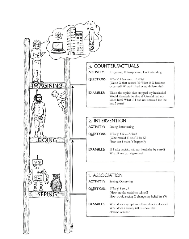
The above “ladder of causation” illustration shows that without a causal model, statistics stay only on the bottom rung of the ladder.
Remember this diagram from above:
Pearl says of it:
John Snow’s painstaking detective work had showed two important things: (1) there is no arrow between Miasma and Water Company (the two are independent), and (2) there is an arrow between Water Company and Water Purity. Left unstated by Snow, but equally important, is a third assumption: (3) the absence of a direct arrow from Water Company to Cholera, which is fairly obvious to us today because we know the water companies were not delivering cholera to their customers by some alternate route. … Because there are no confounders of the relation between Water Company and Cholera, any observed association must be causal. Likewise, since the effect of Water Company on Cholera must go through Water Purity, we conclude (as did Snow) that the observed association between Water Purity and Cholera must also be causal. Snow stated his conclusion in no uncertain terms: if the Southwark and Vauxhall Company had moved its intake point upstream, more than 1,000 lives would have been saved. Few people took note of Snow’s conclusion at the time. He printed a pamphlet of the results at his own expense, and it sold a grand total of fifty-six copies.
I don’t have room to go into the causal language and elegant equations Pearl has in his book, but I’ll mention the ‘do’ operator – the idea of actively changing a cause, as opposed to just observing:
if we are interested in the effect of a drug (D) on lifespan (L), then our query might be written symbolically as: P(L | do(D)). In other words, what is the probability (P) that a typical patient would survive L years if made to take the drug? This question describes what epidemiologists would call an intervention or a treatment and corresponds to what we measure in a clinical trial. In many cases we may also wish to compare P(L | do(D)) with P(L | do(not-D)); the latter describes patients denied treatment, also called the “control” patients. The do-operator signifies that we are dealing with an intervention rather than a passive observation; classical statistics has nothing remotely similar to this operator. We must invoke an intervention operator do(D) to ensure that the observed change in Lifespan L is due to the drug itself and is not confounded with other factors that tend to shorten or lengthen life. If, instead of intervening, we let the patient himself decide whether to take the drug, those other factors might influence his decision, and lifespan differences between taking and not taking the drug would no longer be solely due to the drug. For example, suppose only those who were terminally ill took the drug. Such persons would surely differ from those who did not take the drug, and a comparison of the two groups would reflect differences in the severity of their disease rather than the effect of the drug.
… Note that P(L | D) may be totally different from P(L | do(D)). This difference between seeing and doing is fundamental …A world devoid of P(L | do(D)) and governed solely by P(L | D) would be a strange one indeed. For example, patients would avoid going to the doctor to reduce the probability of being seriously ill; cities would dismiss their firefighters to reduce the incidence of fire…
Pearl notes that we can say that X causes Y if P(Y | do(X)) > P(Y). So here we have a mathematical formula, in his new causal language, for causality!
We could think up other applications for Pearl’s causal diagrams and language. Perhaps indexing of pages by search engines on the internet would benefit by first parsing the causal structure of the story in the document. Perhaps arguments, political or otherwise, could be analyzed to show their causal assumptions.
Pearl says that current convolution nets and deep-learning nets leave out causality. I would mention though that there are also “generative models” that do learn causes. You can test hypotheses about neuronal time-series with a method called “dynamic causal modelling, and in “free energy” based nets, which I mentioned in an earlier blog post, the application of the free energy principle results in a generative model that generates consequences from causes.
But apart from that minor point, I would think the application of Pearl’s causal language and diagrams will give a boost to neural models of all sorts as well as reasoning and logic. His causal diagrams also are easy for a human to understand, unlike the internal weights of recurrent generative nets.
Sources:
Pearl, Judea. The Book of Why: The New Science of Cause and Effect. Basic Books. Kindle Edition.

Leave a comment